Patch-based analysis
NiftyNet is designed to facilitate patch-based medical image analysis. This is implemented with two types of extensible modules:
- Window sampler: sampling image windows from volumes.
- Window aggregator: decoding network’s output windows and the relevant location information, and assembling the volume-level outputs accordingly.
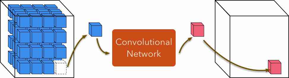
Image window sampling and aggregation.
The relevant configuration parameters are:
- spatial_window_size,
- volume_padding_size,
- border.
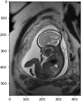
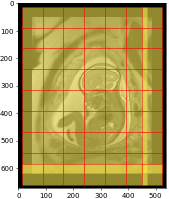
The following sections describes the interaction of these parameters using a slice of fetal MRI as an example.
The code to generate these visualisations is available: NiftyNet/demos.
spatial window size
spatial_window_size defines the spatial size of the input of a
convolutional network (The full shape is jointly determined
by batch size, spatial window size, and number of modalities/channels of the
input volume). The value of spatial_window_size should be less or equal
than the spatial size of all the input files.
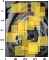
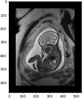
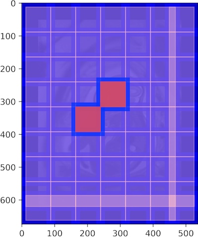
The above figure shows image window sampling locations with:
# in the input source section
spatial_window_size = (100, 100)
from the 574 x 437-pixel MRI, using a uniform window sampler and grid
window sampler respectively.
The uniform window sampler first computes a set of all feasible spatial locations (so that the windows are always within the image) and randomly draws samples from the set.
The grid window sampler extracts all windows from the volume, with minimal
window overlap when the window size is not divisible by the volume size. In
other words, it is running a 100 x 100-pixel sliding window with a step
size of 100 in both spatial dimensions.
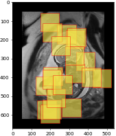
volume padding size
volume_padding_size could be specified at the training and/or inference
stage so that the input volumes are padded and image windows could be sampled
at the borders of the input volume. This is also useful when some of the input
volumes are smaller than the spatial window size.
The follow figure shows image window sampling with the configurations:
# in the input source section
spatial_window_size = (100, 100)

# in the [NETWORK] section
volume_padding_size = (50, 50)
volume_padding_mode = 'constant'
Note that with padding size equals to 50, 50-pixel will be added to both
ends of each dimension, making the new image size: 674 x 537 from (the
original size 574 x 437).
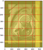
border
This parameter is useful at the inference stage, where a “sliding window” approach is applied to make dense predictions.
If the input and output image windows of a network have the same spatial size,
there is no need for this parameter (`border = 0`) – the window sampler
generates image windows and the corresponding spatial coordinates, the
aggregator reads the coordinate information and assigns the output window to
the output volumes.
However, if by design of the network architecture, a network generates a 76
x 76-pixel prediction when the input size is 100 x 100, we have to adjust
the sampling step of the grid window sampler so that all input spatial
locations get evaluated by the network.
Therefore,
- for the grid window sampler, we would like to have
100 x 100-pixel window generated with a step size of76in both directions; - for the window aggregation, the spatial coordinates of the
76
x 76
-pixel window should be adjusted, for example, from the input’s window coordinates[0, 0, 100, 100]to the output coordinates[12, 12, 88, 88], so that the output window will be concentric with the corresponding input window.
In NiftyNet, both are achieved by setting border size to 12, 12.
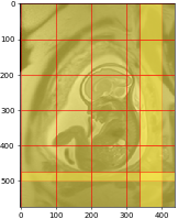
The follow figure shows input image window sampling with the configurations:
# in the input source section
spatial_window_size = (100, 100)

# in the [NETWORK] section
volume_padding_size = (50, 50)
volume_padding_mode = 'constant'

# in the [INFERENCE] section
border = (12, 12)
In the above figure, two of the grid window samples are highlighted (blue) to show the overlap.
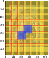
The following figure shows how the 76 x 76 output windows are assigned to
the output volume by the window aggregator.
To confirm the sampling strategy, we visualise the input (blue) and output
(pink) window grids together. The windows are concentric; there is overlap for
the 100 x 100 input windows, but not for the 76 x 76 output windows;
the thickness of the border in between input and output windows is (100 -
76) / 2 = 12 pixels.
Technically, it is possible to automatically determine border when the
network design is known at TF graph construction time. This feature is not
implemented yet (as of Sept. 2018). So the border parameter should be set
manually in the configuration. The formula to compute border is
floor((input size - output size) / 2) for each spatial dimension.
Other features
2.5D windows
Examples in the previous section are in 2-D, but the idea generalises to 3D input:
spatial_window_size = (h, w, d)
will make the sampler to generate 3D windows.
Setting the spatial window size to:
spatial_window_size = (h, w, 1)
will generate 2.5D windows. Using this configuration with random flipping layer during training will effectively use 2.5D input in different views.
Image as window
If all input volume have a consistent size h x w x d, and
in the configuration:
# in the input source section
spatial_window_size = (h, w, d)
The input image will be used as window, i.e., there’s no randomisation when
this configuration is used with the uniform sampler, and only one window sample
per volume when used with the grid sampler.
Multi-channel inputs
The window samples are generated according to the spatial dimensions only.
spatial_window_size, volume_padding_size, and border
accept array values up to three elements.
For multi-channel input images with sizes such as height x width x depth x
num_modalities, the shape of the windows will be
window height x window width x window depth x num_modalities.

